Tree Swallow Life History: R Basics & Data Exploration

This is a tutorial to get you familiar with R and explore ecological concepts through a Tree Swallow nest productivity dataset. Please download the accompanying RMarkdown file and data to follow along with this tutorial in R.

Follow along in RStudio!

For this tutorial, you have the option to follow along online or you can download the R Markdown file and datasets and follow along and practice coding in RStudio. To follow along in RStudio, download the following files:

Download required RMarkdown file

Download required data

Next, you must unzip the folder containing the datasets (TRES) and place the “tree-swallow-dataset.Rmd” R Markdown file into a new folder (e.g. folder name: “R-basics-tutorial”) with the datasets folder (TRES). An example file structure is depicted below:

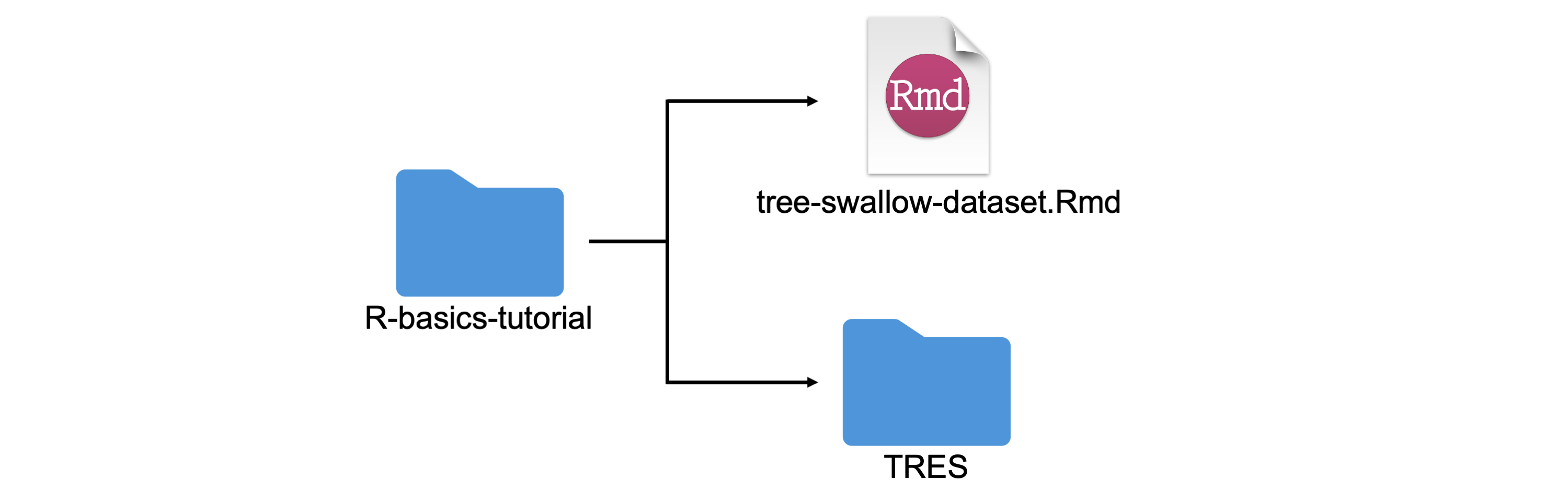
NOTE: in order for this tutorial to run in RStudio, you must follow the file structure above. Your .Rmd file must be labeled “tree-swallow-dataset.Rmd” and the datasets folder must be labeled “TRES”. Make sure you do not use spaces or special characters in your folder name either as good practice!

Tutorial Learning Objectives

In this tutorial you will:

• Explore and utilize basic commands for handling ecological data in R
  • e.g., subsetting, changing class, aggregating data
• Practice graphing data in appropriate formats
  • Graph a simple bar chart
  • Graph a time series
• Observe trends and draw conclusions from figures

Tree Swallow Nest Productivity

Let’s get to know our dataset!

The Tree Swallow (Tachycineta bicolor) is one of the most common birds in eastern North America that normally nests in tree cavities excavated by other species like woodpeckers, but also readily accepts human made nest boxes. Based on this quality and their abundance, Birds Canada has monitored nest boxes of Tree Swallows around the Long Point Biosphere Reserve, Ontario, Canada, from 1974 to 2014. Each summer, volunteer research assistants check nest box contents daily, and band the adults and their young. Nest-box records are available from about 300 boxes from 3-4 sites during this period. Data collected includes nest box observations, clutch initiation dates, clutch size and egg weight, nest success, weather, insect abundance, and banding data. Clutch here refers to the total eggs a bird lays in a nesting attempt. This dataset includes all data entry related to eggs, nests, nestlings, nest check observations, and banding data from 1977 to 2014. More information on this dataset can be found here.

Additionally, in 2021, this dataset was quality checked and made open access by Jonathan Diamond through a Data Rescue internship with the Living Data Project, an initiative through the Canadian Institute of Ecology and Evolution that rescues legacy datasets.

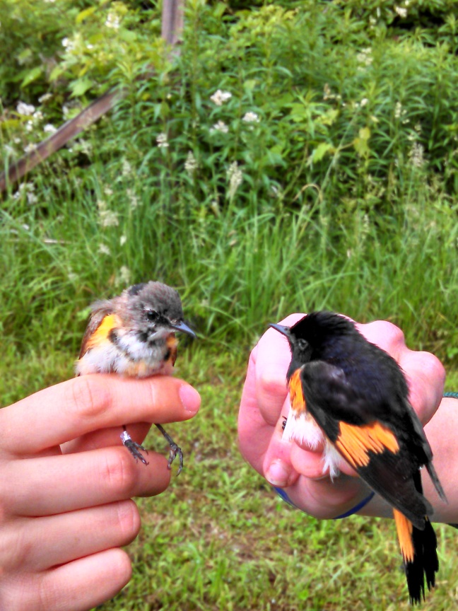
Through Bird Studies Canada, Long Point Bird Observatory monitored three nest box colonies of Tree Swallows.

Tree Swallows utilising a nest box. Photo by Peter Ward. Image from Nature Vancouver.

Bird Banding

Tree Swallows were banded and banding data was recorded. Each band has a unique number so when the bird is recaptured, it is linked to a database that keeps track of the bird overtime. Once the birds were banded, banders collected multiple measurements including species, age, sex, body condition, bird colour, wing length, cord length and mass. For more information on banding, check out this Government of Canada resource that includes descriptions of banding data codes used by the Bird Banding Laboratory.

Check out this video below to see how birds are banded, courtesy of the Monomoy Bird Observatory in Cape Code.

Tree Swallow Age

You might be asking, how can you tell how old a bird is? For the most part, banders rely on the bird’s wing feathers to determine their age. However, after the bird is 2 years old, it’s very difficult to reliably age the birds. Only recapture data can help determine the age of the banded bird after it’s older than 2 years.

Below are age codes used to age birds:

Age Code	Age	Description
JUV	Juvenile	a recently hatched bird, prior to it’s preformative moult
HY	Hatch Year	a bird hatched earlier the same year
AHY	After Hatch Year	a bird hatched in a previous year
SY	Second Year	a bird in its second calendar year
ASY	After Second Year	a bird beyond it’s second year
TY	Third Year	a bird in it’s thrid year
ATY	After Third Year	a bird beyond it’s third year

Installing R

To navigate and complete the following tutorials you will be required to install R and we encourage you to install R Studio.

R is a freely available software and the most recent version of R can be downloaded from: https://cran.r-project.org. After you have installed R, we encourage you to download R Studio as it provides a more user friendly interface to interact with R. R Studio Desktop is freely available from https://rstudio.com/products/rstudio/download/.

The final piece of software that is required for completing the practicals is rmarkdown. Rmarkdown documents weave together narrative text and code to produce formatted, reproducible outputs. If you are unfamiliar with rmarkdown, a short tutorial is available from https://rmarkdown.rstudio.com/articles_intro.html.

Overview of R concepts

In this next section we are going to walk you through a few of the concepts you need to understand in order to work with data in R.

Importing data and packages

In order to work with certain set of data in R, you must first pull them into the program. Before we can pull packages into R, you will first have to install them onto your computer. Run the following code below to download the required packages (without the #s). You only need to install the packages once.

Show code

# install.packages("dplyr")
# install.packages("ggplot2")
# install.packages("tidyr")
# install.packages("lubridate")
# install.packages("reshape")
# install.packages("readr")

Now we can start running those packages by calling on them using the following code:

Show code

library(dplyr)
library(ggplot2)
library(tidyr)
library(lubridate)
library(reshape)
library(readr)
library(distill)

And lastly, we need to pull the actual datasets into R using the read.csv() function, where banding is the name of the object (or in this case datraframe) and the path to the file is within the ().

Show code

banding <- read.csv("TRES/banding_final.csv") #this dataset set contains banding information
nest <- read.csv("TRES/nest_final.csv") #this dataset contains nest information
nestling <- read.csv("TRES/nestling_final.csv") #this dataset contains nestling information

Data Exploration

Let’s do some data exploring! First, let’s see what is in the banding dataset. This will help give us a better idea of what we can look at. Look into the first few rows of the banding dataset. You can do this using the head() function.

Show code

head(banding) # where head() is the function and banding is the dataset

  band_or_recapture band_number sex colour wing_chord wing_flat tail
1                 R    1831.386   F    BLU        116       119   58
2                 R    1881.065   F    BLU        115       119   54
3                 R    2171.200   F    BLU        112       114   55
4                 R    1881.064   M    BLU        123       124   60
5                 B    2351.397   M    BLU        118       119   58
6                 R    1881.042   M    BLU        123       125   56
  p_9 weight       date nest_box age_code year
1  89   22.0 2010-06-01     PT4G      ASY 2010
2  90   19.6 2010-06-01     PT2F      ASY 2010
3  88   21.5 2010-06-01    PT15G      ASY 2010
4  96   21.1 2010-06-01     PT4G      AHY 2010
5  92   22.1 2010-06-01    PT15G      AHY 2010
6  97   20.5 2010-06-01     PT2F      AHY 2010

There are 13 columns in the dataset, each representing a measurement taken when the bird was banded where:

Column Name	Explanation
band_or_recapture	whether the bird has been banded at the time of data entry or previously banded (i.e., has a band already) by B = band and R = recapture
band_number	band number, either from the recaptured birds that already have a band or a new band number
sex	sex of the bird by F = female and M = male
colour	colour of the bird where BLU = blue, BRN = brown, and INT = intermediate
wing_chord	wing_chord measurement in mm
wing_flat	wing_flat measurement in mm
tail	tail measurement in mm
p_9	length of the 9th primary, or the outer primary feather, measured in mm
weight	weight of the bird in grams
date	date the bird was captured recorded as yyyy-mm-dd
nest_box	labeled by site and box number with no spaces
age_code	age of the bird when captured (see previous section for descriptions)
year	year the bird was captured and all above data was collected

You can dig in deeper by using the summary() and str() functions. This is important, because the variables need to match what they are being used for (i.e., to calculate mean, the variable must be numeric (num), not a character (chr), integer (int), or factor (Factor) type).

Show code

# summarise the banding dataset
summary(banding) 

 band_or_recapture   band_number       sex           
 Length:1602        Min.   :1381   Length:1602       
 Class :character   1st Qu.:2312   Class :character  
 Mode  :character   Median :2351   Mode  :character  
                    Mean   :2310                     
                    3rd Qu.:2402                     
                    Max.   :5212                     
    colour            wing_chord      wing_flat          tail      
 Length:1602        Min.   :100.0   Min.   :102.0   Min.   :44.00  
 Class :character   1st Qu.:113.0   1st Qu.:115.0   1st Qu.:53.00  
 Mode  :character   Median :116.0   Median :118.0   Median :55.00  
                    Mean   :115.7   Mean   :117.9   Mean   :54.98  
                    3rd Qu.:118.0   3rd Qu.:121.0   3rd Qu.:57.00  
                    Max.   :129.0   Max.   :130.0   Max.   :69.00  
      p_9             weight          date          
 Min.   : 78.00   Min.   :16.50   Length:1602       
 1st Qu.: 90.00   1st Qu.:19.80   Class :character  
 Median : 92.00   Median :20.50   Mode  :character  
 Mean   : 92.39   Mean   :20.58                     
 3rd Qu.: 95.00   3rd Qu.:21.40                     
 Max.   :109.00   Max.   :25.90                     
   nest_box           age_code              year     
 Length:1602        Length:1602        Min.   :2010  
 Class :character   Class :character   1st Qu.:2011  
 Mode  :character   Mode  :character   Median :2012  
                                       Mean   :2012  
                                       3rd Qu.:2013  
                                       Max.   :2014  

Show code

# check the structure of the banding dataset
str(banding) #This is important, because the variables need to match what they are being used for (i.e., to calculate mean, the variable must be numeric, not a character type)

'data.frame':   1602 obs. of  13 variables:
 $ band_or_recapture: chr  "R" "R" "R" "R" ...
 $ band_number      : num  1831 1881 2171 1881 2351 ...
 $ sex              : chr  "F" "F" "F" "M" ...
 $ colour           : chr  "BLU" "BLU" "BLU" "BLU" ...
 $ wing_chord       : num  116 115 112 123 118 123 110 111 112 117 ...
 $ wing_flat        : num  119 119 114 124 119 125 112 113 114 118 ...
 $ tail             : num  58 54 55 60 58 56 55 52 55 54 ...
 $ p_9              : int  89 90 88 96 92 97 89 87 90 92 ...
 $ weight           : num  22 19.6 21.5 21.1 22.1 20.5 20 21.6 19.8 20.5 ...
 $ date             : chr  "2010-06-01" "2010-06-01" "2010-06-01" "2010-06-01" ...
 $ nest_box         : chr  "PT4G" "PT2F" "PT15G" "PT4G" ...
 $ age_code         : chr  "ASY" "ASY" "ASY" "AHY" ...
 $ year             : int  2010 2010 2010 2010 2010 2010 2010 2010 2010 2010 ...

Subsetting and conditional subsetting elements

• The [ operator can be used to select multiple elements of an object: The [ operator can be used to extract specific rows or columns from a dataset where DATA[row, column]

• The $ operator can be used to extract elements by the element’s name

Let’s try pulling the first row from the banding dataset

Show code

banding[c(1),] #notice how there is a comma after c(1)? This specifies we want to subset the first row!

  band_or_recapture band_number sex colour wing_chord wing_flat tail
1                 R    1831.386   F    BLU        116       119   58
  p_9 weight       date nest_box age_code year
1  89     22 2010-06-01     PT4G      ASY 2010

Let’s make a mini version of our banding dataset, and call it banding2, by subsetting rows 1 through 50 and columns 2, and 5 through 13

Show code

banding2 <- banding[c(1:50), c(2,5:13)] #where banding2 is our new dataframe containing data from rows 1:50 and columns 2 and 5:13 from the banding dataset. 

Applying different functions to data

You can also run functions on different variables of your datasets which you can select by using $. You can wrap these in different functions to calculate various things. For example, let’s try calculating the mean weight from our banding2 dataset and assign it to a new variable called mean_weight. The following line of code creates a column in banding2 called mean_weight and assigns the mean of the column weight from banding2 to it. Then use the head() function to take a quick look.

Show code

banding2$mean_weight <- mean(banding2$weight)

head(banding2)

  band_number wing_chord wing_flat tail p_9 weight       date
1    1831.386        116       119   58  89   22.0 2010-06-01
2    1881.065        115       119   54  90   19.6 2010-06-01
3    2171.200        112       114   55  88   21.5 2010-06-01
4    1881.064        123       124   60  96   21.1 2010-06-01
5    2351.397        118       119   58  92   22.1 2010-06-01
6    1881.042        123       125   56  97   20.5 2010-06-01
  nest_box age_code year mean_weight
1     PT4G      ASY 2010      20.815
2     PT2F      ASY 2010      20.815
3    PT15G      ASY 2010      20.815
4     PT4G      AHY 2010      20.815
5    PT15G      AHY 2010      20.815
6     PT2F      AHY 2010      20.815

What if we wanted to calculate the mean weight of the Tree Swallows as recorded in the banding dataset based on their sex? We could do that by grouping how we calculate the mean by using the aggregate() function. The aggregate function can work to group data as follows:

aggregate(y ~ a + b + c + …, df, mean)

Where y is the variable you want to take the mean of, a, b, c… are variables that you are interested in grouping these means by, df is the dataframe that you are pulling these data from, and mean is instructing the command that the summary statistic you want to complete is the mean. Lets try it out!

Show code

# If we wanted to look at the average weight of female and male birds in the banding dataset we would use aggregate() like this
banding3 <- aggregate(weight ~ sex, banding, mean) # banding3 is where these values will be stored
banding3

  sex   weight
1   F 20.41623
2   M 20.75646

---

Try coding

# Try looking at the mean weight of Tree Swallows grouped by sex and year, call this new data frame 'banding4'

Show code

# Answer
# banding3 <- aggregate(weight ~ sex, year, mean)

Logical operators

Now that you have a good handle on basic subsetting, let’s dig a little deeper and use logical operators to further subset your data.

What if you want to focus in on looking at just one sex? How would you extract only data related to female birds from these data? One way to do this would be to use the subset() function and logical operators to separate out the data of interests from your dataset.

• < (less than)
• <= (less than or equal to)
• > (greater than)
• >= (greater than or equal to)
• == (exactly equal to)
• != (not equal to)
• x | y (x OR y)
• x & y (x AND y)

It is important to note that certain logical operators only work on certain classes of data. For example, if we looked at sex (class of factor) we can’t subset values that are less than or equal to Female (this would make no sense since Female is not a number or integer!).

Show code

# pull out female birds from your banding dataset 
head(subset(banding, sex == "F")) #the head function limits the amount of rows displayed

  band_or_recapture band_number sex colour wing_chord wing_flat tail
1                 R    1831.386   F    BLU        116       119   58
2                 R    1881.065   F    BLU        115       119   54
3                 R    2171.200   F    BLU        112       114   55
7                 B    2351.397   F    BLU        110       112   55
8                 R    2321.083   F    BLU        111       113   52
9                 B    2351.397   F    INT        112       114   55
  p_9 weight       date nest_box age_code year
1  89   22.0 2010-06-01     PT4G      ASY 2010
2  90   19.6 2010-06-01     PT2F      ASY 2010
3  88   21.5 2010-06-01    PT15G      ASY 2010
7  89   20.0 2012-06-01     PT1J      ASY 2010
8  87   21.6 2012-06-01     PT4J      ASY 2010
9  90   19.8 2012-06-01     PT8K      AHY 2010

Remember, if you want to store this in a df to look at later I would have to assign it to a vector called “female_birds”.

Notice how the vector female_birds changed from 853 observations to 495 observations?

---

Try coding

# Try to subset a dataframe called 'male_birds' that consists of male birds with the chord_length less than or equal to 150

Show code

# Answer
# male_birds <- subset(banding, sex == "M" & chord_length <= 150)

---

Question

How many male birds have a chord_length less than or equal to 150?

Show code

# Answer = 749

---

Graphing basics

Having fun yet? I know I am! Let’s look at the basics of a plot.

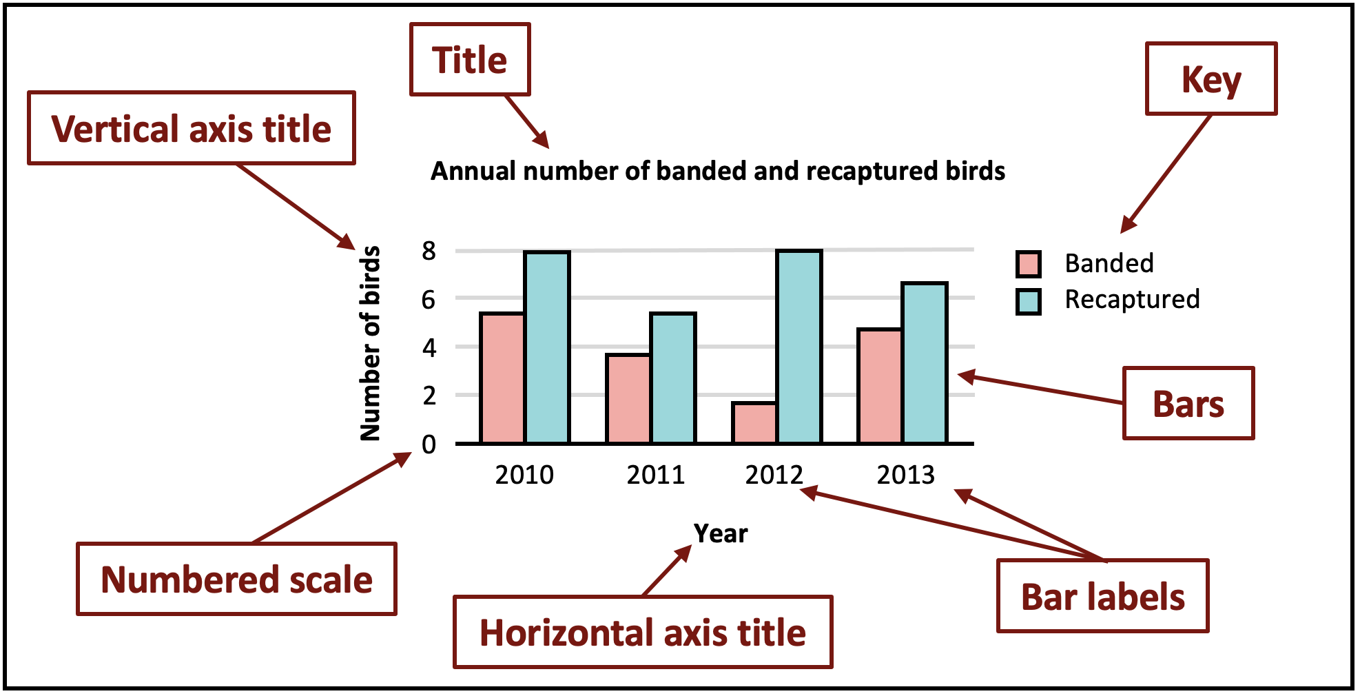
Now that we are refreshed in the elements of a graph, let’s graph a relatively simple bar plot with our banding data frame.

Let’s look at the number of banded and recaptured birds there were each year. We will use ggplot to visualize the data.

Show code

# First, we will create a table base on the band_or_recapture column and the year column
tbl1 <- with(banding, table(band_or_recapture, year))  
tbl1

                 year
band_or_recapture 2010 2011 2012 2013 2014
                B   62  125  118   68  101
                R  179  264  292  139  254

Show code

# Next, we can plot our table 
ggplot(as.data.frame(tbl1), aes(x =factor(year), y = Freq, fill = band_or_recapture))+ #we've changed the format of our table to a dataframe so we can plot it. 
  geom_col(position = 'dodge') #geom_column is the type of graph, and position='dodge' allows us to visualize the barplots side by side.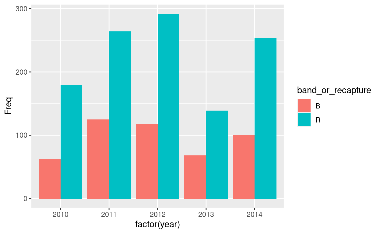

Congrats! You’ve made your first graph. We can change elements of the graph by adding labels and titles, changing the theme and colours of our bars.

Show code

# Add labels and change colours
ggplot(as.data.frame(tbl1), aes(x =factor(year), y = Freq, fill = band_or_recapture))+ 
  geom_col(position = 'dodge') +
  xlab('Year') +
  ylab('Number of birds') +
  scale_fill_manual(name= "Banded or Recaptured", values=c("B" = 'lightskyblue', "R" = 'plum3'))+
  ggtitle("Birds banded or recaptured from 2010-2014") +
  theme_classic() #gets rid of grey background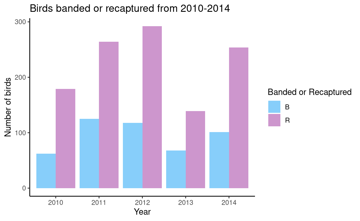

(If you’d like to learn more about ggplot, this tutorial is great!)

---

Question

What trends do you see?

Why do you think there are more recaptured birds compared to banded birds every year?

---

More data exploration

Next, let’s change gears and take a quick look at the egg nestling dataset.

# Lets get a sense of what columns are present in our dataset
head(nestling)

  nest_box band_number year clutch_number day_1_weight day_12_weight
1     PT7F  2351.39972 2014            NA         <NA>          <NA>
2     PT7F  2351.39973 2014            NA         <NA>          <NA>
3     PT7F  2351.39974 2014            NA         <NA>          <NA>
4    PT14G  2351.39975 2014            NA         <NA>          <NA>
5    PT14G  2351.39976 2014            NA         <NA>          <NA>
6    PT14G  2351.39977 2014            NA         <NA>          <NA>
  site nest_code
1 <NA>      <NA>
2 <NA>      <NA>
3 <NA>      <NA>
4 <NA>      <NA>
5 <NA>      <NA>
6 <NA>      <NA>

# Lets look at the structure of our new dataframe, nestling:

str(nestling)

'data.frame':   32536 obs. of  8 variables:
 $ nest_box     : chr  "PT7F" "PT7F" "PT7F" "PT14G" ...
 $ band_number  : chr  "2351.39972" "2351.39973" "2351.39974" "2351.39975" ...
 $ year         : int  2014 2014 2014 2014 2014 2014 2014 2014 2014 2014 ...
 $ clutch_number: int  NA NA NA NA NA NA NA NA NA NA ...
 $ day_1_weight : chr  NA NA NA NA ...
 $ day_12_weight: chr  NA NA NA NA ...
 $ site         : chr  NA NA NA NA ...
 $ nest_code    : chr  NA NA NA NA ...

Show code

#We don't have entries for all rows of our dataframe. They will appear as **NA**s. We see the weight is a character vector. Let's change that to numeric using the as.numeric() function. Let's start #with the **day_1_weight** column:

nestling$day_1_weight <- as.numeric(nestling$day_1_weight)

# Now the **day_12_weight** column:

nestling$day_12_weight <- as.numeric(nestling$day_12_weight)


# Lets look at the structure of our new dataframe, nestling again:
str(nestling)

'data.frame':   32536 obs. of  8 variables:
 $ nest_box     : chr  "PT7F" "PT7F" "PT7F" "PT14G" ...
 $ band_number  : chr  "2351.39972" "2351.39973" "2351.39974" "2351.39975" ...
 $ year         : int  2014 2014 2014 2014 2014 2014 2014 2014 2014 2014 ...
 $ clutch_number: int  NA NA NA NA NA NA NA NA NA NA ...
 $ day_1_weight : num  NA NA NA NA NA NA NA NA NA NA ...
 $ day_12_weight: num  NA NA NA NA NA NA NA NA NA NA ...
 $ site         : chr  NA NA NA NA ...
 $ nest_code    : chr  NA NA NA NA ...

We want to summarize our data so we can calculate the mean of each weight by year.

nestling_weight <- nestling %>%
  group_by(year) %>% # groups weights by year
  filter(is.na(day_1_weight) == F,  #gets rid of NAs
         is.na(day_12_weight) == F) %>%
  summarise(mean_day_1 = mean(day_1_weight), #calculates the mean of each year 
            mean_day_12 = mean(day_12_weight)) 

# NOTE" '%>%' is known as a pipe operator in R, it helps pass the output of one function 
# as an input to another function to make coding easier and more efficient

# We can convert the mean weights to long format, which gives us a weight column,
# with both weight variables, and a total column which contains the weights

nestling_weight2 <- gather(nestling_weight, weight, total, mean_day_1:mean_day_12)

#Look at the structure of our new dataframe, nestling_weight2

str(nestling_weight2)

tibble [74 × 3] (S3: tbl_df/tbl/data.frame)
 $ year  : int [1:74] 1977 1978 1979 1980 1981 1982 1983 1984 1985 1986 ...
 $ weight: chr [1:74] "mean_day_1" "mean_day_1" "mean_day_1" "mean_day_1" ...
 $ total : num [1:74] 21.83 1.76 1.69 2.18 2.03 ...

Ok, now we can plot it using ggplot.

Show code

ggplot(data = nestling_weight2,
       aes(x = year, y = total, group = weight)) + #Year goes on the x axis, weight(totals) on the y axis, and we group by each the means of each day
  geom_line(aes(linetype = weight, color = weight)) + #aes changes the aesthetics of the lines so that linetype and colors are different from each other
  theme_classic()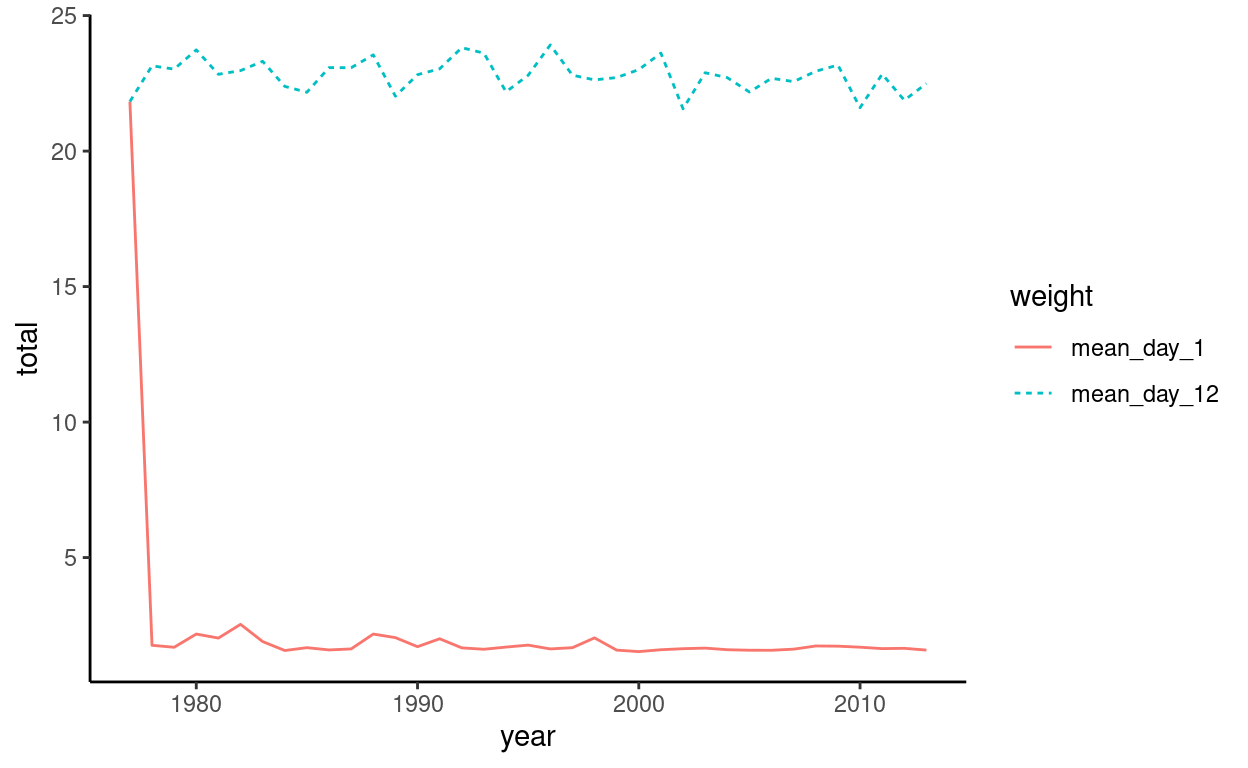

Hmm, looks like something is not quite right in our plot. There seems to be an outlier within the data. If we assume this is a data entry error, we can get rid of it. Since it looks like an earlier date, let’s just look at the first few rows (n = 10) and see if we can find the outlier.

Show code

head(nestling_weight2, n = 10)

# A tibble: 10 × 3
    year weight     total
   <int> <chr>      <dbl>
 1  1977 mean_day_1 21.8 
 2  1978 mean_day_1  1.76
 3  1979 mean_day_1  1.69
 4  1980 mean_day_1  2.18
 5  1981 mean_day_1  2.03
 6  1982 mean_day_1  2.54
 7  1983 mean_day_1  1.90
 8  1984 mean_day_1  1.57
 9  1985 mean_day_1  1.68
10  1986 mean_day_1  1.59

Ah ha! The first row contains a mean_day_1 weight of 21.8. This is likely an error. Let’s get rid of it and then re-plot it.

Show code

nestling_weight2 <- nestling_weight2[-1,]
ggplot(data = nestling_weight2,
       aes(x = year, y = total, group = weight)) + #Year goes on the x axis, weight(totals) on the y axis, and we group by each the means of each day
  geom_line(aes(linetype = weight, color = weight)) + #aes changes the aesthetics of the lines so that linetype and colors are different from each other
  theme_classic()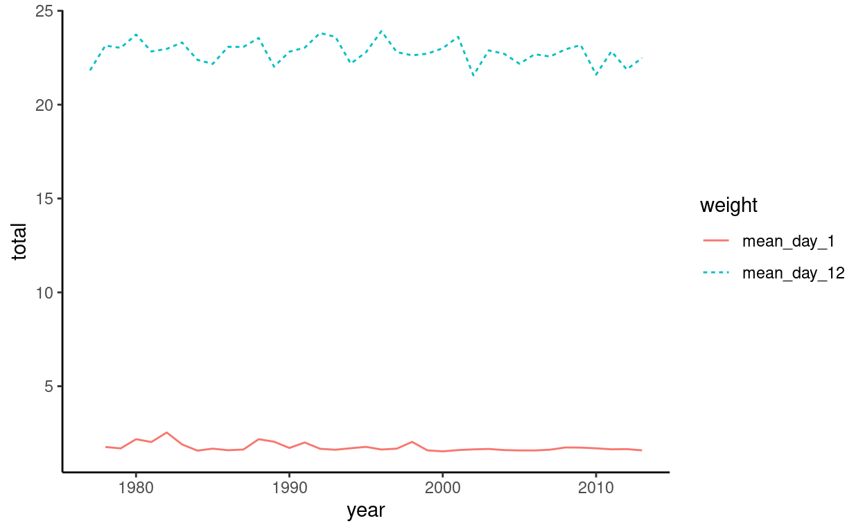

Much better!

---

Questions

Do you see any trends within this datasets over time?

What other variables could you look at within the nestling dataset?

---

Next Steps

You have completed the “Getting familiar with R and the Tree Swallow Dataset” tutorial!

Looking for more of a challenge? Check out this tutorial where we use the Tree Swallow Dataset to examine ecological concepts like life history traits and sexual dimorphism.

Check out this cool video on nesting Tree Swallows!